Introduction
Cointegration testing remains one of the most applied testing procedures in econometrics. Introduced in 1983 by Sir W Granger (Granger, 1983) and Engle and Granger (1987), many testing procedures have been developed. There are the residual-based tests of the null of no cointegration, the most popular being the Engle-Granger (1987) approach and the Phillips-Ouliaris (1990) approach. Both the Engle-Granger and the Phillips-Ouliaris approaches are inbuilt in Eviews as a group object. The difference between the two is that while autocorrelation is corrected by allowing for the lags of the dependent variable in the Engle-Granger approach (which is the ADF approach applied on the residuals from the single-equation bivariate model), in the Phillips-Ouliaris approach, autocorrelation is dealt with non-parametrically with the test based on bias-corrected autocorrelation coefficient and standard error.One of the problems of testing for cointegration is the presence of structural breaks in the data generating process. The fact is that structural break can seriously mess up the result as the test statistics will often fail to reject unit root because they have low power when structural break is present. To illustrate, the Engle-Granger framework for testing for cointegration is actually the testing for unit root under null using the ADF test statistic. This test will fail to reject the null of unit root, while the PP, assuming the null of stationarity, will fail to reject the alternative hypothesis of unit root. The problem is that the introduction of a structural break into the process gets the ADF test statistic confused. Let \(y_t\) and \(x_t\) be two unit-root processes with a one-time break in \(y_t\):\[\begin{align*} y_t=&y_{t-1}+\epsilon_{1t}+DUM_t\\ x_t=&x_{t-1}+\epsilon_{2t}\end{align*}\]In the first process, we have both the stochastic and the deterministic trends, the latter being a result of the break. We can integrate the first expression to have\[y_t=y_0+\sum_{j=1}^t\epsilon_{1j}+\sum_{j=1}^tDUM_{j}=y_0+\sum_{j=1}^t\epsilon_{1j}+DUM\cdot t\]The impulse has cumulated into a trend, more like something perpetual riding on time factor itself. The second process is made up of the initial value as well as the stochastic trend, i.e.,
\[x_t=x_0+\sum_{j=1}^t\epsilon_{2j}\]Suppose we regress \(y_t\) on \(x_t\). More specifically, the following residuals are generated \(\hat{u}_t=y_t-\hat{\beta} x_t\). Is \(\hat{u}_t\) stationary so we can ascertain the cointegration between \(y_t\) and \(x_t\)? The answer is no. To see why, we rewrite \(\hat{u}_t\) as\[\hat{u}_t=\left(y_0+\sum_{j=1}^t\epsilon_{1j}+DUM\cdot t\right)-\hat{\beta} \left(x_0+\sum_{j=1}^t\epsilon_{2j}\right)\]Rearranged and taxonomized, this expression becomes: \(\hat{u}_t\) as\[\hat{u}_t=\underset{I(0)}{\underbrace{y_0- \hat{\beta}x_0}}+\underset{I(1)}{\underbrace{DUM\cdot t}}+\underset{I(0)}{\underbrace{\left(\underset{I(1)}{\underbrace{\sum_{j=1}^t\epsilon_{1j}}}-\underset{I(1)}{\underbrace{\hat{\beta} \sum_{j=1}^t\epsilon_{2j}}}\right)}}\]Each of the cumulated terms in the bracket is I(1) and their linear combination is I(0). Thus, for \(u_t\) to be I(0) and guarantee stationarity of the residuals and, by so doing, establish cointegration between \(y_t\) and \(x_t\), the term \(DUM\cdot t\) must be set to zero. Indeed, this term is I(1). Thus, without accounting for breaks in the process, both ADF and PP statistics will wrongly accept unit root hypothesis. We therefore failed to establish cointegration between two I(1) variables, whose linear combination would be stationary but for the presence of structural breaks. In sum, structural breaks induces non-stationarity.
The question now is: how do we detect structural breaks in cointegrated relation? A number of test statistics have been proposed to formally integrate structural breaks into cointegration. A retest of many macroeconomic variables previously found to have unit roots has confirmed that indeed those variables are stationary after accounting for breaks. This suggests persistence or permanence in these variables is a result of breaks and not inherent.
Four approaches to accommodating structural breaks in cointegration will be discussed:
Six model specifications are investigated. They are termed \(i=A_n, A, B, C, D, E\) and are given by\[y_t=\begin{cases}\Gamma_i(t)+x_t^\prime\beta+\epsilon_t,&{i=A_n, A, B, C}\\\Gamma_i(t)+x_t^\prime\beta_0+x_t^\prime\beta_1DU_t+\epsilon_t,&{i=D, E} \end{cases}\]where\[\begin{cases}\Gamma_{A_n}(t)=\alpha+\theta DU_t\\\Gamma_A(t)=\alpha+\zeta t+\theta DU_t\\\Gamma_B(t)=\alpha+\zeta t+\theta DT_t\\\Gamma_C(t)=\alpha+\zeta t+\theta DU_t+\gamma DT^*_t\\\Gamma_D(t)=\alpha+\theta DU_t\\\Gamma_E(t)=\alpha+\zeta t+\theta DU_t+\gamma DT^*_t\end{cases}\]The dummy variables in the model are constructed as\[DU_t=\begin{cases}1,&\forall t>TB\\0,&otherwise\end{cases}\]and\[DT^*_t=\begin{cases}t-TB,&\forall t>TB\\0,&otherwise\end{cases}\]The first dummy \(DU_t\) is a level shift dummy while \(DT_t^*\) cumulates the effect of the one-off break (impulse) in the data after the break at point \(TB\).
\[x_t=x_0+\sum_{j=1}^t\epsilon_{2j}\]Suppose we regress \(y_t\) on \(x_t\). More specifically, the following residuals are generated \(\hat{u}_t=y_t-\hat{\beta} x_t\). Is \(\hat{u}_t\) stationary so we can ascertain the cointegration between \(y_t\) and \(x_t\)? The answer is no. To see why, we rewrite \(\hat{u}_t\) as\[\hat{u}_t=\left(y_0+\sum_{j=1}^t\epsilon_{1j}+DUM\cdot t\right)-\hat{\beta} \left(x_0+\sum_{j=1}^t\epsilon_{2j}\right)\]Rearranged and taxonomized, this expression becomes: \(\hat{u}_t\) as\[\hat{u}_t=\underset{I(0)}{\underbrace{y_0- \hat{\beta}x_0}}+\underset{I(1)}{\underbrace{DUM\cdot t}}+\underset{I(0)}{\underbrace{\left(\underset{I(1)}{\underbrace{\sum_{j=1}^t\epsilon_{1j}}}-\underset{I(1)}{\underbrace{\hat{\beta} \sum_{j=1}^t\epsilon_{2j}}}\right)}}\]Each of the cumulated terms in the bracket is I(1) and their linear combination is I(0). Thus, for \(u_t\) to be I(0) and guarantee stationarity of the residuals and, by so doing, establish cointegration between \(y_t\) and \(x_t\), the term \(DUM\cdot t\) must be set to zero. Indeed, this term is I(1). Thus, without accounting for breaks in the process, both ADF and PP statistics will wrongly accept unit root hypothesis. We therefore failed to establish cointegration between two I(1) variables, whose linear combination would be stationary but for the presence of structural breaks. In sum, structural breaks induces non-stationarity.
The question now is: how do we detect structural breaks in cointegrated relation? A number of test statistics have been proposed to formally integrate structural breaks into cointegration. A retest of many macroeconomic variables previously found to have unit roots has confirmed that indeed those variables are stationary after accounting for breaks. This suggests persistence or permanence in these variables is a result of breaks and not inherent.
Four approaches to accommodating structural breaks in cointegration will be discussed:
- the Carrion-i-Silvestre-Sansó (Carrion-i-Silvestre and Sansó, 2006) approach.
- the Gregory-Hansen approach (Gregory and Hansen, 1996a,b),
- the Hatemi-J (2008) approach, and
- the Arai-Kurozumi (2007) approach
The Carrion-i-Silvestre-Sansó (Carrion-i-Silvestre and Sansó, 2006) approach
In this post, we'll focus on the Carrion-i-Silvestre-Sansó (Carrion-i-Silvestre and Sansó, 2006) approach. There are basically two variants of the the Carrion-i-Silvestre-Sansó test, which depends on whether the regressors in the model are strictly exogenous or not. In each case, there are six specifications.
- Strict Exogeneity of the Regressors
Six model specifications are investigated. They are termed \(i=A_n, A, B, C, D, E\) and are given by\[y_t=\begin{cases}\Gamma_i(t)+x_t^\prime\beta+\epsilon_t,&{i=A_n, A, B, C}\\\Gamma_i(t)+x_t^\prime\beta_0+x_t^\prime\beta_1DU_t+\epsilon_t,&{i=D, E} \end{cases}\]where\[\begin{cases}\Gamma_{A_n}(t)=\alpha+\theta DU_t\\\Gamma_A(t)=\alpha+\zeta t+\theta DU_t\\\Gamma_B(t)=\alpha+\zeta t+\theta DT_t\\\Gamma_C(t)=\alpha+\zeta t+\theta DU_t+\gamma DT^*_t\\\Gamma_D(t)=\alpha+\theta DU_t\\\Gamma_E(t)=\alpha+\zeta t+\theta DU_t+\gamma DT^*_t\end{cases}\]The dummy variables in the model are constructed as\[DU_t=\begin{cases}1,&\forall t>TB\\0,&otherwise\end{cases}\]and\[DT^*_t=\begin{cases}t-TB,&\forall t>TB\\0,&otherwise\end{cases}\]The first dummy \(DU_t\) is a level shift dummy while \(DT_t^*\) cumulates the effect of the one-off break (impulse) in the data after the break at point \(TB\).The test statistic is based on \(SC_i(\lambda)=T^{-2}\omega_1^{-2}\sum_{t=1}^TS_{it}^2\) where \(S_{it}=\sum_{j=1}^t\hat{\epsilon}_{ij}\) and \(\omega_1=T^{-1}\sum_{t=1}^T\hat{\epsilon}_t^2+2\sum_{j=1}^{lq}\omega_j\sum_{t=j+1}^T\hat{\epsilon}_t^\prime\hat{\epsilon}_{t-j}\) is the Newey-West nonparametric estimator of the long-run variance of \(\hat{\epsilon}_t\) with \(\omega_j=1-j/(lq+1)\) as the weight on all autocovariances and indicating the more distant autocovariances are the less their weights in the computation of long-run variance. This statistic is a ratio of two variances and as such can be referred to F-statistic. However, there is a presence of nuisance parameter, the break point, with which the statistic varies. To overcome this problem, Carrion-I-Silvestre and Sansó (2006) employ a Monte Carlo simulation to construct a set of critical values reported in their paper.
2. Non-Strict Exogeneity of the Regressors
For the case where the regressors are not strictly exogenous, Carrion-i-Silvestre and Sansó (2006) propose to use one of the approaches suggested by Phillips and Hansen (1990), Saikkonen (1991), and Stock and Watson (1993) to obtain an efficient estimation of the cointegrating vectors. We adopt the DOLS in this implementation and it's given by\[y_t=\begin{cases}\Gamma_i(t)+x_t^\prime\beta+\sum_{j=-k}^{k}\Delta x_{t-j}^\prime\gamma_j +\epsilon_t,&{i=A_n, A, B, C}\\\Gamma_i(t)+x_t^\prime\beta_0+x_t^\prime\beta_1DU_t+\sum_{j=-k}^{k}\Delta x_{t-j}^\prime\gamma_j+\epsilon_t,&{i=D, E} \end{cases}\] \(SC_i^+(\lambda)=T^{-2}\omega_1^{-2}\sum_{t=1}^T(S_{it})^{2+}\) where \(S_{it}^+=\sum_{j=1}^t\hat{\epsilon}_{ij}\)
Eviews addin
The following addin is for implementing the method for non-strictly exogenous regressors with unknown break dates. The break date estimated is one and this is in line with the objective of the Carrion-i-Silvestre-Sanso objective (Ensure you go through their paper as well). I may consider the other case for strictly exogenous variables later. The data used for this example can be sourced here.
The addin is straightforward to use. The figure below shows the spool object saving the graph and the table for the results.

Figure 1
In Figure 2, similar results have been presented. The difference is that Model E has been used and the pre-whitened results have also been included.
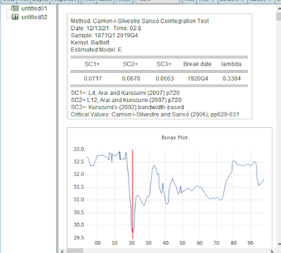

Figure 3
Figure 3 shows the dialog box. You can make your options as you deem appropriate. For example, you can choose any of the methods as shown in Figure 4. Also note that the critical values are not reported. Interested person can see the paper by the authors of the method. Meanwhile, for this method, Carrion-i-Silvestre and Sanso only report the critical values for up to 4 exogeneous variables. Nevertheless, the addin allows you to carry out text for model having more than four exogeneous variables.

Figure 4
The criterion in the dialog box is used to select the optimal numbers for leads/lags.
In the next posts, on cointegration with structural breaks, we shall be looking at all the remaining 3 methods.
If you find this addin helpful, drop a message or better still follow!!!
From here, a big thank-you to you.
© 2021 Olayeni Olaolu Richard. Originally published 12/13/2021


