Blog Archive

Showing posts with label addin. Show all posts

Friday, December 31, 2021

Unit root test with partial information on the break date

Introduction

Partial information on the location of break date can help improve the power of the test for unit root under break. It is this observation that informs the unit root testing under a local break-in trend by Harvey, Leybourne, and Taylor (2013) where the authors employ partial information on the break date. It builds on the insight first projected by Andrews (1993), who observed that prior information about the location of the break will help even if the analysts do not have full information about the precise break date.

The setback of most of the unit root tests that allow for breaks is that they lose their power if there is no such break compared to the tests that do not account for such break in the first place. Yet another issue with the procedure for detecting break dates is that when the break dates are not large enough there is tendency that they will not be detected. Undetected breaks when they are present can lead to loss of power in this case even for the tests that do not allow for such break. It then means that testing for unit root under breaks must be carefully sorted out.

In short the idea is to employ restricted search and this involves searching within the domain of the break where it is more likely for the break to have occurred. The benefit of this restricted search is that uncertainty around the break point reduces should there be a break point there indeed. The improvement in power as a result therefore means that the test should not fail to reject when it should.


HLT Approach

Harvey, Leybourne and Taylor (2013), in pursing this objective, adopted the Perron-Rodríguez (2003) approach employing the GLS-based infimum test because of its superior power. It is found that the GLS-based infmum tests perform better among those tests that do not allow for break detection and has greater robustness among those that allow for it. To robustify this approach, they proposed the union of rejections strategy. The union of rejections strategy attempts to derive power from the two discreet worlds, in which case the strategy pools the power inherent in the restricted-range with-trend break and the without-trend break unit roots. Using this strategy, the null of unit root is rejected 

if either the restricted-range with-trend break infimum unit root test or the without-trend break unit root test rejects.

In this way, there is no need for prior break date detection, which in itself can compromise the power of the test. 


Model

We can begin our review of this method by stating the following DGP:\[\begin{align*}y_t=&\mu+\beta t+\gamma_T DT_t (\tau_0)+u_t, \;\; t=1,\dots,T\\ u_t=&\rho_T u_{t-1}+\epsilon_t  \;\; t=2,\dots,T\end{align*}\]where \(DT_t(\tau)=1(t>[\tau T])(t-[\tau T])\). The null hypothesis is \(H_0:\rho_T=1\) against the alternative that \(H_c:\rho_T=1-c/T\) where \(c>0\). A crucial assumption which features in the computation of the asymptotic critical value is that the trend break magnitude is local-to-zero so that uncertainty can be captured, that is, \(\gamma_T=\kappa\omega_\epsilon T^{-1/2}\) with \(\kappa\) is a constant. 

The Procedure to Computing the Union of Rejections

To construct the union of rejections decision rule, the steps are involved have been broken down to a couple of blocks.
  • STEP 1: The following sub-steps are involved: 
      1. Assume there is a known break date at \(\tau T\), where \(\tau\in(0,1)\). The data are first transformed as:\[Z_{\bar{\rho}}=[y_1,y_2-\rho y_1,\dots,y_T-\rho y_{T-1}]^\prime\] and \[Z_{\bar{\rho},\tau}=[z_1,z_2-\rho z_1,\dots,z_T-\rho z_{T-1}]^\prime\]where \(z_t=[1,t,DT_t(\tau)]^\prime\) and \(\bar{\rho}=1-\bar{c}/T\) with \(\bar{c}=17.6\);
      2. Apply the LS regression on the transformed data in Step 1 and obtain the residuals \(\tilde{u}_t=y_t-\tilde{\mu}-\tilde{\beta} t-\tilde{\gamma} DT_t (\tau)\). The GLS estimates for \(\theta\), \(\tilde{\theta}=(\tilde{\mu},\tilde{\beta},\tilde{\gamma})\), are\[\tilde{\theta}=\underset{\theta}{\text{argmin}}\; u_t^\prime u_t;\]
      3. The ADF is applied to the residuals obtained in Step 2:\[\Delta \tilde{u}_t=\hat{\pi} \tilde{u}_{t-1}+\sum_{j=1}^k\hat{\psi}_j\Delta\tilde{u}_{t-j}+\hat{e}_t.\]
  • STEP 2: Instead of assuming a known break date, HLT make use of the infimum GLS detrended Dickey-Fuller statistic as follows:
      1. Define the window mid-point parameter \(\tau_m\) and the window width parameter \(\delta\);
      2. Define the search window as\[\Lambda(\tau_m,\delta):=[\tau_m-\delta/2,\tau_m+\delta/2]\]and, if \(\tau_m-\delta/2<0\) or \(\tau_m+\delta/2>1\), then define the following respectively \(\Lambda(\tau_m,\delta):=[\epsilon,\tau_m+\delta/2]\) or \(\Lambda(\tau_m,\delta):=[\tau_m-\delta/2,1-\epsilon]\), where \(\epsilon\) is a small number set to 0.001.
      3. Then compute \[MDF(\tau_m,\delta):=\underset{\tau\in\Lambda(\tau_m,\delta)}{\text{inf}}DF^{GLS}(\tau)\]which amounts to repeating the sub-steps Step 1 for every observation corresponding to the fraction defined in the restricted window \(\Lambda(\tau_m,\delta)\) and finding the least DF statistic 
  • STEP 3: The Elliot et al (1996) DF-GLS is carried out as follows:
      1. The data are first transformed as in Step 1 in the procedure above without including the break date and with \(\bar{c}=13.5\);
      2. Apply the LS regression on the transformed data in Step 1 and obtain the residuals \(\tilde{u}_t^e=y_t-\tilde{\mu}-\tilde{\beta} t\). The GLS estimates for \(\theta\), \(\tilde{\theta}=(\tilde{\mu},\tilde{\beta})\), are\[\tilde{\theta}=\underset{\theta}{\text{argmin}}\; u_t^{e\prime} u_t^e;\]
      3. The ADF is applied to the residuals obtained in Step 2:\[\Delta \tilde{u}^e_t=\hat{\pi} \tilde{u}_{t-1}^e+\sum_{j=1}^k\hat{\psi}_j\Delta\tilde{u}_{t-j}^e+\hat{e}_t.\]
      4. The DF-GLS statistic is the t-value associated with \(\hat{\pi}\) and is denoted \(DF^{GLS}\)
  • STEP 4: The union of rejections strategy involves the rejection of the null of unit root, as stated early, 

if either the restricted-range with-trend break infimum unit root test or the without-trend break unit root test rejects.

The decision rule is therefore given by\[U(\tau_m,\delta):=\text{Reject} \;H_0 \;\text{if}\;\left\{DF^{GLS}_U(\tau_m,\delta):=\text{min}[DF^{GLS},\frac{cv_{DF}}{cv_{MDF}}MDF(\tau_m,\delta)]<\lambda cv_{DF}\right\}\]where \(cv_{DF}\) and \(cv_{MDF}\) are the associated critical values and \(\lambda\) is a scaling factor. The critical values \(cv_{DF}\) are reported in Elliot et al (1993) and those of \(cv_{MDF}\) are reported in HLT (2013). The critical values for the scaling factor are also reported in Table 2 of HLT (2013).


Eviews addin

For the purpose of implementing this test seamlessly, I have developed an addin in Eviews. As usual, the philosophy of simplicity has been emphasized. Like the inbuilt unit root tests, the addin has been latched on the series object. This means it is a menu in the time series object's add-ins. To have it listed as seen in Figure 1, you must install the addin. 

In Figure 1, I subject LINV series to HLT unit root. 

Figure 1


The following dialog box presents you with options to choose from. The lag selection criteria include the popular ones such as the Akaike, Schwarz and Hanna-Quinn as well as their modified versions. Additionally, there is the t-statistic for optimal lag length selection. Significance levels indicates the choices for the level of significance for the lag length. The window width and the widow mid-point are also presented and you can also choose them as appropriate. The trimming can become too extreme sometimes. Under this circumstance, you are likely to express errors, whereby the addin will issue error message to inform you appropriately. This is likely going to be the case if the number of observations is too small.

The prior break date edit box can be left empty if there is no such date to be considered. Yet, The window width  and mid-point can be adjusted. A diffuse prior can be expressed with large value of window width. Lower values of window width suggests that the analyst expresses more certainty about the mid-point. For example, if the window width \(\delta=0.050\) is combined with \(\tau_m=0.50\) it means the analyst expresses more conviction that the break date happens around the mid point of the data than when he combines the width \(\delta=0.200\) with the same mid-point.

Figure 2

The output is presented in Figure 3. According to Equation 4 in HLT, one has to compare DF-GLS-U with the corresponding \(\lambda\)-scaled critical value denoted as Lam-sc'd c.v. In case the DF-GLS-U values are less than the Lam-sc'd c.v., then the null hypothesis of unit root is rejected. In this example, the DF-GLS-U are higher than those for Lam-sc'd c.v. Thus, the null hypothesis near unit root is not rejected.

Figure 3

Lastly, if there are reasons to choose a break date around which there is a doubt, this can be entered as a prior date break. In Figure 4, I enter 1976Q1 as the break date and then express the extent of my doubt around this date by selecting the window width as 0.05. 

Figure 4

Compared to window width of 0.200, this is a lot more precisely expressed. Thus, it is no surprise that the break date is found in the neighborhood of the putative break date. This can be seen in Figure 5. 

Figure 5

Happy New Year everyone. Let moderation be your guiding principle as you go out to celebrate the new year. 💥💥💥

Friday, December 24, 2021

Bootstrap ARDL: Eviews addin

Introduction

Let's quickly wrap our heads around the idea of bootstrap ARDL by first looking at the concept of weak exogeneity. The idea is better understood within the VECM approach. Suppose there are two variables of interest in that they are both endogenous. It means we can model them jointly. Recall that in the VECM system of equations, each equation has two parts to it: the short-run (in differences) and the long-run (in levels). The long-run component is a linear combination of the lagged endogenous variables plus some deterministic terms, and the effects are the "loading" factors that convey the impact of this linear combination to the changes in each of the endogenous variables. They are also called the speed of adjustments as they reveal how the short-run adjustment takes place due to the disequilibrium in the long-run component. Long-term feedbacks are therefore through the loading factors. If the loading factor for a particular equation in the system is negligible, then long-term feedback may well be set to zero and we say the particular endogenous variable is weakly exogenous. When endogenous variables are weakly exogenous, the system can be simplified into two sub-models: the conditional and the marginal models. We can then focus on the conditional model, that is, the model whose loading factors are significant, and ignore the marginal model. It all means we have less number of parameters to estimates because the number of equations too has been reduced. 

If you understand the preceding, then you already know the make up of ARDL. In this sense, the dynamic regressors in ARDL are considered weakly exogenous. The model analyzed is termed conditional. A telltale of being a conditional model is the first difference at "lag 0" often included for the regressors, (such as \(\varphi_0^\prime \Delta x_t\) in the following model), and should remind the user that the model employed is conditional; otherwise, it's unconditional:\[\Delta y_t = \alpha+\theta t+\rho y_{t-1} +\gamma^\prime x_{t-1}+\sum_{j=1}^{p-1}\phi_j \Delta y_{t-j}+\varphi_0^\prime \Delta x_t+\sum_{j=1}^{q-1}\varphi_j^\prime \Delta x_{t-j}+\epsilon_t\]Thus in models where the users rotate the dependent variables, this assumption of weak exogeneity of the exogenous variables is being violated.

While weak exogeneity assumption is being violated, especially when authors implicitly assume that the variables can be rotated such that the same variable is being used as a dependent variable in one estimation and as an independent variable in another, the degenerate cases are also common (the degenerate cases are discussed here). The first of these degenerate cases arises when the joint test (F statistic) of the lagged dependent and independent variables is significant and the t-statistic on the lagged dependent variable is significant as well while the F statistic  of the lagged independent variable(s) is not significant. The recommended solution to the lagged dependent degenerate case is to formulate the model such that the dependent variable is I(1). Here again, users also violate this assumption by not ensuring that the dependent variable is I(1).

Added to these issues is the inconclusiveness in bounds testing. How do we decide whether cointegration exists or not if the computed F-statistic falls within the lower and the upper bounds? As is well known, the critical values provided by PSS, or Narayan or even by Sam, McNown and Goh do not provide a clear roadmap on what the decision must be. Experience often shows that the case of fractionally integrated process, \(x_t=\sum_{j=1}^t\Delta ^{(d)}_{t-j}\xi_j\), where \(d\in(-0.5,0.5)\cup(0.5,1.5)\) and \(\Delta_t^{(d)}:=\Gamma(t+d)/\Gamma(d)\Gamma(t+1)\) cannot be ruled out. In other words, series occasionally don't fall perfectly into I(0) or I(1).

To proceed, we can bootstrap. This approach works because no parametric assumptions are made about the distribution. Rather data are allowed to speak. Therefore, through bootstrap a data-based distribution emerges that can be used for making decisions. 


The algorithm used...

The bootstrap steps used in this add-in are as follows, where I'm working with the hypothesis that the model is trend-restricted in a bivariate model, that is, \(H_0:\theta_1=\rho_1=\gamma_1=0\) (You can read more about the five model specifications in PSS here): 

    1. Imposing the null hypothesis, e.g., \(H_0:\theta_1=\rho_1=\gamma_1=0\), estimate the restricted model: \[\begin{align*}\Delta y_t =& \alpha_1+\theta_1 t+\rho_1 y_{t-1} +\gamma_1 x_{t-1}+\sum_{j=1}^{p_y-1}\phi_{j,1} \Delta y_{t-j}+\sum_{j=0}^{q_y-1}\varphi_{j,1} \Delta x_{t-j}+\epsilon_{1,t}\\\Delta x_t =& \alpha_2+\theta_2 t+\rho_2 y_{t-1} +\gamma_2 x_{t-1}+\sum_{j=1}^{p_x-1}\phi_{j,2} \Delta y_{t-j}+\sum_{j=0}^{q_x-1}\varphi_{j,2} \Delta x_{t-j}+\epsilon_{2,t}\end{align*}\]and obtain the residuals \(\hat{\epsilon}_{1,t}\) and \(\hat{\epsilon}_{2,t}\). Note that this system needs not be balanced as the orders may not necessarily be the same;
    2. Obtain the centered residuals \(\tilde{\epsilon}_{i,t}=(\hat{\epsilon}_{i,t}-\bar{\hat{\epsilon}}_{i,t})\);
    3. Resample \(\tilde{\epsilon}_{i,t}\) with replacement to obtain \(\epsilon^*_{i,t}\)
    4. Using the model in Step 1, evaluating the system at the estimated values, generate pseudo-data (bootstrap data): \(y_t^*\) and \(x_t^*\), which can be recovered as \(y_t^*=y_{t-1}^*+\Delta y_t^*\) and ditto for \(x_t^*\);
    5. Estimate unrestricted model using the bootstrap data:\[\Delta y_t^* = \tilde{\alpha}_1+\tilde{\theta}_1 t+\tilde{\rho}_1 y_{t-1}^* +\tilde{\gamma}_1 x_{t-1}^*+\sum_{j=1}^{p_y-1}\tilde{\phi}_{j,1} \Delta y_{t-j}^*+\sum_{j=0}^{q_y-1}\tilde{\varphi}_{j,1} \Delta x_{t-j}^*\]
    6. Test the necessary hypothesis: \(H_0:\tilde{\theta}_1=\tilde{\rho}_1=\tilde{\gamma}_1=0\);
    7. Repeat the steps in 3 to 6 B times (say, B=1000).

Eviews addin

The implementation has been synced to addin, which I prefer to working through all these steps each time. You can obtain the addin here. To use it, you just need to estimate your ARDL model as usual. All the 5 specifications in Eviews can be bootstrapped. After estimation of the model, click on the Proc tab of the estimated model and hover to Add-ins for ARDL equation object. The Bootstrap ARDL menu should be located provided it has already been installed.

Figure 1 shows the Bootstrap ARDL addin dialog box. Although the details of the choices that can be made are self-explaining, the coefficient uncertainty deserves some comments. Usually, the bootstrap is carried out at the estimated values of the parameters. While this is innocuous, the "right" thing to do, in my opinion, is to sample from the distributions of the parameters thereby incorporating the fact that they have not been precisely estimated. To give the user this choice, I have included the Check option for Coefficient uncertainty. 

Figures 2 to 5 give different results of the same model under different choices. I think this should available for sensitivity study of the results. In this output, I have appended -F or -t to indicate the F or t statistic.

Figure 1: Bootstrap ARDL Dialog Box


Figure 2: Sample output


Figure 3: Sample output


Figure 4: Sample output


Figure 5: Sample output

Suggestions are welcome. 

Saturday, December 18, 2021

Fractional Frequency Flexible Fourier Form ARDL: A Demonstration

Introduction

This method has been applied in three known published papers. They're all published between 2020 and 2021 and this is suggestive of the future boom of this approach. It's therefore important that we discuss it here. I'll be discussing the estimation part of this method in this post. The other part, which involves bootstrap, will be discussed in a subsequent post. 

Let's delve into it at once. Why this kind of formulation? Yes, the economy goes through a lot of changes mostly in the short run. But long-run changes also take place rather smoothly and unnoticeably. Modelling smooth, slow and steady changes in the economic relation is a profitable venture in policy analysis. The Fourier flexible form is a good methodological proposition for this modelling. Even so, some changes are not smooth even in the long run. Violent changes do take place. Wars. All manners of pandemic. Benign, beneficial and nevertheless sudden changes also do take place. Ushering in a new regime of democratically elected office holders often signals the enthronement of rules of law and a good bait to the investors, who come with new technologies that eventually reset the path of long-term outcomes in the economy. These changes too, though not smooth, can still be efficiently captured by Fourier form. Earlier discussants of this modelling strategy include Gallant, Davies, Becker, Enders, Li in their various publications. Omay joins the train by introducing the fractional frequency idea, which was extended by Olayeni, Tiwari and Wohar to long T panel. Other ideas of modelling slow changes are due to Bierens and co-authors, who propose the Chebyshev approximation. 

The method 

All that I want to show you is how to implement this model using the ARDL method in Eviews. First, I will invite you to read one of the previous posts in this blog, where I have briefly discussed the ARDL method. (Read about it here.) More importantly, the section, ARDL at a Glance will be helpful. Pay attention to Cases 1 and 2 under the model specifications. I further invite you to read about the bootstrap method here. In this post, we are going to apply the knowledge of bootstrap. Consider the following model, which I call FARDL(p,q):\[\Delta y_t=\theta+d(t)+\rho y_{t-1}+\gamma x_{t-1} +\sum_{j=1}^{p-1}\psi_j\Delta y_{t-j}+\sum_{j=0}^{q-1}\varphi_j\Delta x_{t-j}+\epsilon_t\]where\[d(t)=\sum_{k=1}^n\alpha_k\text{cos}\left(\frac{2\pi k t}{T}\right)+ \sum_{k=1}^n\beta_k\text{sin}\left(\frac{2\pi k t}{T}\right)\]To estimate this model, a couple of practical issues are involved that you will need to sort out very early. The first is the choice of the frequency. At what frequency will the estimation be conducted? Trivial as it might appear, it has implications for the results. The second is the number of Fourier terms to be included. In the generic specification given above, the number of terms is set to \(n\). In a more serious study, this has to be determined too. Most often, the selection criteria are used for this purpose and the goal is to selected the value that minimizes the criterion used. I will assume these two issues are already sorted out and what remains is to proceed to estimation. In line with the approach employing fractional frequency, one frequency parameter will be used. However, we'll grid-search for its optimal value. Thus, we state as follows, setting \(n=1\):\[d(t)=\alpha\text{cos}\left(\frac{2\pi k t}{T}\right)+\beta\text{sin}\left(\frac{2\pi k t}{T}\right)\]

Fractional frequency

In most studies it may be instructive to find the fractional frequency rather than arbitrarily impose a particular integer frequency. The reason is that the integer frequency imposed may well not be supported by the data. Therefore, it is crucial to find the frequency that delivers the optimal value in terms of the information criterion so chosen. Finding the optimal fractional frequency itself deserves some note.  In this section, I give a thorough discussion of one way this optimal value can be found. First, I present the snippet of the code that does that. Get the code here. Subsequently, I explain what the snippet does and how it does it. 

Code snippet... 


Here is the code to find the fractional frequency parameter value: 
  1. matrix(1000,2) matrixAIC=na
  2. !c=1
  3. for !k=0.1 to 4 step 0.01
    • equation fourierardl.ardl lcons lincome @ cos(2*@pi*!k*@obsnum/@obssmpl) sin(2*@pi*!k*@obsnum/@obssmpl)
    • matrixAIC(!c,2)=fourierardl.@aic
    • matrixAIC(!c,1)=!k
    • !c=!c+1
  4. next
  5. vector minvecAIC=@cimin(matrixAIC)
  6. !indexminAIC=minvecAIC(2)
  7. scalar kstar=matrixAIC(!indexminAIC,1)


...and the explanation

What this code snippet does is to find the value of the frequency, \(k^*\), that minimizes the Akaike Information Criterion (AIC). You can change this to any of the other criteria (@schwarz or @hq). The first line, Line 1, declares the matrix object as the storage. The order is obviously more than what is needed but does not pose any problem since I set that to na. I need a counter and it is declared in Line 2. In Line 3, a for-next-step loop is initialized. This is complemented by Line 4. Every command issued within this loop will not only be carried out, it will be repeated 391 times, with the values of \(k\) incrementing \(0.1, 0.11,0.12,\dots,3.99,4.00\). By default, that is, without step included in Line 3, the integer values will be assumed. Since we need a fine grid, over which we want to search, we reduce the step to \(0.01\) on each iteration. 

The commands within the loop need to be explained. The first bullet declares an equation object named fourierardl and assigns ARDL method to it. ardl refers to the second model specification already discussed in a post here. Thus, the command says the model should estimated without including the trend specification at all. Therefore, without the fixed regressors included, the specification would simply read

        equation fourierardl.ardl lcons lincome @

However, to include the Fourier flexible form terms in the model, we treat them as fixed regressors and they are placed just immediately after @-sign:

         @ cos(2*@pi*!k*@obsnum/@obssmpl) sin(2*@pi*!k*@obsnum/@obssmpl) 

This means the Fourier flexible form terms are to be treated as fixed regressors in the estimation.

Next, we need the associated AIC. It is an equation data member and can be accessed as declared in the second bullet. The AIC value at the iteration !c is grabbed and stored in the first column of matrixAIC. The corresponding frequency parameter value is likewise stored in the second column of matrixAIC. The last bullet within the loop is the counter initialized at Line 2. It is being incremented by 1 just to ensure what has been stored previously is not overwritten. Otherwise, it will be zero-work done! So pay attention to such little things.

Immediately outside the loop (well, I call it post-loop section), we need to find one of those 391 frequency parameter values corresponding to the least of the 391 AIC values. One way to do this is to first identify the index of the least AIC value. The matrix utility function @cimin() achieves that for us. It gives us the index of the least value in each column of a matrix. In this case, it will return the 2 indices of the least values, the first for the first column and the other for the second column. For a newbie, here is a lurking slippery source of error. The index so identified in the first column should not be given a hoot. This is because the second element in the second column is the least and the index will read 1. This is not what we want. We want the value of \(k\), call it \(k^*\), that corresponds to the least value of AIC. If you don't get this point, you can open the vector minvecAIC and examine the elements. I'm pretty sure, the value in the first entry will be 1 and always 1!

Then how do we select the corresponding value of the frequency parameter? We need to first grab the index of the least AIC. Since the values of AIC are stored in the second column, the index must be the second element in minvecAIC. It is selected by issuing minvecAIC(2), with 2 indicating the second element in minvecAIC. I assign it to a scalar !indexminAIC in Line 6. Now, finally, in Line 7, I select the coveted value of frequency parameter. The command  scalar kstar=matrixAIC(!indexminAIC,1)says look up the value in Row !indexminAIC and Column 1. Remember the frequency parameters are in the second column.

Optimal fractional frequency


In Figure 1, we present the graph of the optimal fractional frequency. It is observed immediately that the value of the frequency parameter that achieves the minimal AIC is 2.78. There is no way we would have known this had we not grid searched as we did in the preceding section. This figure is the graphical representation of the elements in matrixAIC and has been plotted using xy-line graph so that we have AIC on the y-axis and k on the x-axis. The vertical dashed line is a marker of the the optimal value located at point 2.78 on the x-axis. You can also add this to your work to lend credence to its worth.

Having gone this far, the question is: what next?

Figure 1: Optimal frequency

Yes, what next?


Yes the next thing is the FARDL estimation. But if you have been following closely, you will have noticed we've already done so for 391 regressions. One of them, which must be reported, is what we are looking for here. And that is the one that corresponds to the optimal frequency just found in the section above. We are not going to estimate 391 regression models again. Rather, we only need to plug in the optimal frequency parameter and estimate just one regression model. That model is the FARDL we are looking for. Let's do it together. You already savvy about what to do, ehn? Since the optimal frequency parameter, \(k^*\), is already in the workfile, it means you can use it in subsequent computations. Let's use point-and-click approach at this point. 

Figure 2 shows what we should be doing. Note in particular the scalar for the frequency parameter. It is now the optimal one:

Figure 2: What FARDL dialog box should look like

Figure 3 shows the results of this estimation, a FARDL(2,0). The output from this estimation can be analyzed as usual. As shown in Figure 4, we can carry out the bounds testing. 

Figure 3: FARDL Output


Figure 4: Bounds testing


What about carrying out the Augmented FARDL? Of course, that too is possible. Just use the Augmented ARDL addin for this; it can be found here

FYI: If you already installed the old version of this addin, released prior to this post, you might need to download the new one again and reinstall it. Only the updated version of this addin is guaranteed to handle this augmented bounds testing for Fourier ARDL without a glitch.

Figure 5: Augmented Bounds Testing

Figure 6: Testable Form for the FARDL

The current augmented addin also produces an OLS version of the long-run form useful in its own right as shown in Figure 6. In subsequent post, this will come in handy. Therefore, in this post, no further comment on why it's important. 

If this helps, just hit the follow button.👉😉😏 I will hear load and clear. Thank you.


Wednesday, December 15, 2021

Conducting Augmented ARDL in Eviews Using Addin

Introduction

The Augmented ARDL is an approach designed to respond to the question of whether or not the dependent variable should be either I(0) or I(1). With I(0) as the dependent variable, it is difficult to infer long-run relationship between the dependent variable and the regressor(s) even if the F-statistic is above upper critical bound in the well used bounds-testing procedure. The reason is that, in the event that the I(0) is used as the dependent variable, the series will necessarily be stationary (Permit my tautological rigmarole)! This means in jointly testing for long-run relationship via F statistic, the fact that the computed F value is above the upper bound might just reflect the I(0)-ness of the dependent variable. What is more? Other exogenous variables may turn out to be insignificant, suggesting without testing the I(0) dependent variable along with them, the resulting t statistic (if there is only one exogenous variable) or F statistic (if there are more than one exogenous variable) becomes insignificant. Thus, the I(0) variable in the joint relationship may dominate whether or not other variables are significantly contributing to the long-run relationship. The result is always wrong inference.

ARDL at a glance

While the PSS-ARDL approach is a workhorse for estimating and testing for long-run relationship under the joint occurrence of I(0) and I(1) variables, there are certain assumptions the applied researchers often take for granted thereby violating the conditions necessary for using the PSS-ARDL in the first place. For a bivariate specification, the PSS-ARDL(p,q), in its most general form, is given by\[\Delta y_t=\alpha+\beta t+\rho y_{t-1}+\gamma x_{t-1}+\sum_{j=1}^{p-1}\delta_j\Delta y_{t-j}+\sum_{j=0}^{q-1}\theta_j\Delta x_{t-j} +z_t^\prime\Phi+\epsilon_t\]where \(z_t\) represents the exogenous variables and could contain other deterministic variables like dummy variables and \(\Phi\) is the vector of the associated parameters. Based on this specification, Pesaran et al., (2001) highlight five different cases for bounds testing, each informing different null hypothesis testing.  Although some of them are less interesting because they have less practical value, it is instructive to be aware of them:

        • CASE 1: No intercept and no trend
        • CASE 2: Restricted intercept and no trend
        • CASE 3: Unrestricted intercept and no trend
        • CASE 4: Unrestricted intercept and restricted trend
        • CASE 5: Unrestricted intercept and unrestricted trend

Intercept or trend is restricted if it is included in the long-run or levels relationship. For each of these cases, Pesaran et al., (2001) compute the associated t- and F-statistic critical values. These critical values are reported in that paper and readers are invited to consult the paper to obtain the necessary critical values (if you want since these values are reported pro bono). 

The cases above correspond to the following restrictions on the model:
  • CASE 1: The estimated model is given by \[\Delta y_t=\rho y_{t-1}+\gamma x_{t-1}+\sum_{j=1}^{p-1}\delta_j\Delta y_{t-j}+\sum_{j=0}^{q-1}\theta_j\Delta x_{t-j} +z_t^\prime\Phi+\epsilon_t\] and the null hypothesis is \(H_0:\rho=\gamma=0\). This model is recommended if the series have been demeaned and/or detrended. Absent these operations, it should not be used for any analysis except the researcher is strongly persuaded that it is the most suitable for the work or simply for pedagogical purposes.
  • CASE 2: The estimated model is \[\Delta y_t=\alpha+\rho y_{t-1}+\gamma x_{t-1}+\sum_{j=1}^{p-1}\delta_j\Delta y_{t-j}+\sum_{j=0}^{q-1}\theta_j\Delta x_{t-j} +z^\prime_t\Phi+\epsilon_t\]where in this case \(\beta=0\). The null hypothesis \(H_0:\alpha=\rho=\gamma=0\). The restrictions imply that both the dependent variable and the regressors are moving around their respective mean values. Think of the parameter \(\alpha\) as \(\alpha=-\rho\zeta_y-\gamma\zeta_x\), where \(\zeta_i\) are the respective mean values or the steady state values to  which the variables gravitate in the long run. Substituting this restriction into the model, we have \[\Delta y_t=\rho(y_{t-1}-\zeta_y)+\gamma (x_{t-1}-\zeta_x)+\sum_{j=1}^{p-1}\delta_j\Delta y_{t-j}+\sum_{j=0}^{q-1}\theta_j\Delta x_{t-j} +z^\prime_t\Phi+\epsilon_t\]This model therefore possesses some practical values and is suitable for modelling the behaviour of some variables in the long run. However, because the dependent variable do not possess the trend due to the absence of intercept in the short run, this specification's utility is limited given that most economic variables are I(1).
  • CASE 3: The estimated model is the same as in CASE 2 with \(\beta=0\). However, \(H_0:\rho=\gamma=0\). This implies the intercept is pushed into the short-run relationship and it means the dependent variable has a linear trend,  trending upwards or downwards depending on the direction dictated by \(\alpha\). This characteristic is benign if the dependent variable is really having the trend in it. However, this is not a feature of I(0) dependent variable. As most macroeconomic variables are I(1), this specification is often recommended. In Eviews, it's the default setting for model specification.
  • CASE 4: The model estimated for CASE 4 is the full model. Here, trend is restricted while the intercept is unrestricted. The null hypothesis is therefore  \(H_0:\beta=\rho=\gamma=0\). This specification suggests that the dependent variable is trending in the long run. If, in the long run, the dependent variable is not trending, it means this specification might just be a wrong choice to model the dependent variable.
  • The last case where both the intercept and the trend are unrestricted is a perverse description of the macroeconomic variables. It is a full model but it means the dependent variable is trending quadratically. This does not fit most cases and is rarely used. The null hypothesis is  \(H_0:\rho=\gamma=0\).
The F statistic and the associated t statistic for bounds testing are reported in PSS. 

Getting More Gist about ARDL from ADF

The F statistic for bounds testing referred to above is necessary, but it is not sufficient, to detect whether or not there is long run relationship between the dependent variable and the regressors. The reason for this is the presence of both I(0) and I(1) and their treatment as the dependent variable in the given model. Note that one of the requirements for valid inference about the existence of cointegration between the dependent and the regressors is that the dependent variable must be I(1). We can get the gist of this point by looking more closely at the relationship between the ARDL and the ADF model. You may be wondering why the dependent variable must be I(1) in the ARDL model specification. The first thing to observe is that ARDL is a multivariate formulation of the augmented Dickey Fuller (ADF). Does that sound strange? 

Suppose \(H_0: \gamma=\theta_0=\theta_1=\cdots=\theta_q=0\), that is, the insignificance of other exogenous variables in the model, cannot be rejected. Then the model reduces to the standard ADF. From this, we can see that if \(\rho\) is significantly negative, stationarity is established. If this is the case, variable \(y_t\) will be reckoned as I(0). Thus, the ADF is given by\[\Delta y_t=\alpha+\rho y_{t-1}+\sum_{j=1}^{p-1}\delta_j\Delta y_{t-j}+\epsilon_t\]The fact that \(y_t\) is stationary at levels means that \(\rho\) must be significant whether or not the coefficients on other variables are significant. Therefore, in a test involving this I(0) variable as a dependent variable and possibly I(1) as independent variable(s), and where the coefficient on the latter is found to be insignificant, it's still possible to find cointegration not because there is one between these variables, but because the significance of the (lag of) dependent variable dominates the joint test and because only a subset of the associated alternative hypothesis is being considered. This is what the bounds testing does without separating the significance of \(\rho\) and \(\gamma\). Note that F test for bounds testing is based on the joint significance of these parameters. However, the joint test of \(\rho\) and \(\gamma\) does not tell us about the significance of \(\gamma\).

Degenerate cases

How then can we proceed here? More tests needed. To find out how, we must first realize what the issues are really like in this case. At the center of this are the two cases of degeneracy. They arise because the bounds testing (a joint F test) involves both the coefficient on the lagged dependent variable \(\rho\) in the model above and the coefficients of lagged exogenous variables. Although PSS reported the t statistic for \(\rho\) separately with a view to having robust inference, not only do the researchers often ignore it, the t statistic so reported along with the F statistic is not enough to avoid the pitfall. In short, the null hypothesis for the bounds testing \(H_{0}: \rho=\gamma=0\) can be seen as a compound one involving  \(H_{0,1}: \rho=0\) and \(H_{0,2}: \gamma=0\). So rejection of either is not a proof of cointegration. This is because the alternative is not just \(H_{0}: \rho\neq\gamma\neq 0\) as often assumed in application; the alternative instead involves \(H_{0,1}: \rho\neq0\) and \(H_{0,2}: \gamma\neq0\) as well. In other words, a more comprehensive hypothesis testing procedure must involve the null hypotheses of these alternatives. Thus, we have the following null hypotheses:
        1. \(H_{0}: \rho=\gamma= 0\), and \(H_{1,1}: \rho\neq0\), \(H_{1,2}: \gamma\neq0\) 
        2. \(H_{0,1}: \rho=0\) and \(H_{1,1}: \rho\neq0\)
        3. \(H_{1,2}: \gamma=0\) and \(H_{1,2}: \gamma\neq0\) 

Taxonomies of Augmented Bounds Test 

Therefore, we state the following taxonomy for testing hypothesis:
      • if the null hypotheses (1) and (2) are not rejected but (3) is, we have a case of degenerate lagged independent variable. This case implies absence of cointegration;
      • if the null hypotheses (1) and (3) are not rejected but (2) is, we have a case of degenerate lagged dependent variable. This case also implies absence of cointegration; and
      • if the null hypotheses (1), (2) and (3) are rejected, then there is cointegration 
We now have a clear roadmap to follow. What this implies is that one needs to augment the testing as stated above. Hence the augmented ARDL testing procedure. With this procedure for testing for cointegration, it is no longer an issue whether or not the dependent variable is I(0) or I(1) as long as all the three null hypotheses are rejected.

Now the Eviews addin...

First note that this addin has been written in Eviews 12. Its functionality in lower version is therefore not guaranteed. 

Using Eviews for testing this hypothesis should be straightforward but may be laborious. Eviews can help you here. All that is needed is reporting all the three cases noted above as against the two cases reported in Eviews. The following addin helps you with all the computations you might need to do. 

To use it, just estimate your ARDL model as usual and then use the Proc tab to locate the add ins. In Figure 1, we have the ARDL method environment. Two variables are included. I choose the maximum lag of eight because I have enough quarterly data, 596 observations in total.

Figure 1

Once the model is estimated, use the Proc tab to locate Add-ins as shown in Figure 2 

Figure 2

Click on Augmented ARDL Bound Test and you will have the figure referred to in Figure 3. The tests are reported underneath what you see here. Just scroll down to look them up.


Figure 3

Figure 4


What is shown in Figure 4 should be the same as reported natively by Eviews. The addition that has been appended by this addin is the Exogenous F-Bounds Test shown in Figure 5. For the confirmation of the test, we append the Wald test for exogenous variables in the spool. It comes under the title exogenous_wald_table. You can click to view it.

Figure 5

In this example, we are sure of cointegration because all the three computed statistics are above the upper bound, suggested no case of degeneracy is lurking in our results.

Note the following...

Before working on the ARDL output, be sure to name it. At the moment, if the output is UNTITLED, Error 169 will be generated. The glitch is a really slippery error. It will be corrected later. 

The results have the fill of the existing table for bounds testing in Eviews but have been appended with the tests for the exogenous variables. The F statistic is used for testing the exogenous variables. Thus, we have the section for Overall F-Bounds Test which is the Null Hypothesis (1) above; the section for the t-Bounds Test which is the Null Hypothesis (2); and, the section for the Exogenous F-Bounds Test which is the Null Hypothesis (3). The first two of these sections should be the same as in the native Eviews report. The last is an addition based on the paper by Sam, McNown and Goh (2018).  

From the application point of view, in this case, the Exogenous F-Bounds test for Cases 2 and 3 are the same:
  • CASE 2: Restricted intercept and no trend
  • CASE 3: Unrestricted intercept and no trend
  •  just as Cases 4 and 5 are the same:

  • CASE 4: Unrestricted intercept and restricted trend
  • CASE 5: Unrestricted intercept and unrestricted trend
  • Therefore, the same critical values are reported for them in the literature. Thus, in the Eviews addin the long run for both cases are reported. 

    The link to the addin is here. The data used in this example is here.

    Thank you for reading a long post😀.

    Sunday, December 12, 2021

    Cointegration Tests Under Structural Breaks (Part I)

    Introduction

    Cointegration testing remains one of the most applied testing procedures in econometrics. Introduced in 1983 by Sir W Granger (Granger, 1983) and Engle and Granger (1987), many testing procedures have been developed. There are the residual-based tests of the null of no cointegration, the most popular being the Engle-Granger (1987) approach and the Phillips-Ouliaris (1990) approach. Both the Engle-Granger and the Phillips-Ouliaris approaches are inbuilt in Eviews as a group object. The difference between the two is that while autocorrelation is corrected by allowing for the lags of the dependent variable in the Engle-Granger approach (which is the ADF approach applied on the residuals from the single-equation bivariate model), in the Phillips-Ouliaris approach, autocorrelation is dealt with non-parametrically with the test based on bias-corrected autocorrelation coefficient and standard error.

    One of the problems of testing for cointegration is the presence of structural breaks in the data generating process. The fact is that structural break can seriously mess up the result as the test statistics will often fail to reject unit root because they have low power when structural break is present. To illustrate, the Engle-Granger framework for testing for cointegration is actually the testing for unit root under null using the ADF test statistic. This test will fail to reject the null of unit root, while the PP, assuming the null of stationarity, will fail to reject the alternative hypothesis of unit root. The problem is that the introduction of a structural break into the process gets the ADF test statistic confused. Let \(y_t\) and \(x_t\) be two unit-root processes with a one-time break in \(y_t\):\[\begin{align*} y_t=&y_{t-1}+\epsilon_{1t}+DUM_t\\ x_t=&x_{t-1}+\epsilon_{2t}\end{align*}\]In the first process, we have both the stochastic and the deterministic trends, the latter being a result of the break. We can integrate the first expression to have\[y_t=y_0+\sum_{j=1}^t\epsilon_{1j}+\sum_{j=1}^tDUM_{j}=y_0+\sum_{j=1}^t\epsilon_{1j}+DUM\cdot t\]The impulse has cumulated into a trend, more like something perpetual riding on time factor itself. The second process is made up of the initial value as well as the stochastic trend, i.e.,
    \[x_t=x_0+\sum_{j=1}^t\epsilon_{2j}\]Suppose we regress \(y_t\) on \(x_t\). More specifically, the following residuals are generated \(\hat{u}_t=y_t-\hat{\beta} x_t\). Is \(\hat{u}_t\) stationary so we can ascertain the cointegration between \(y_t\) and \(x_t\)? The answer is no. To see why, we rewrite \(\hat{u}_t\) as\[\hat{u}_t=\left(y_0+\sum_{j=1}^t\epsilon_{1j}+DUM\cdot t\right)-\hat{\beta} \left(x_0+\sum_{j=1}^t\epsilon_{2j}\right)\]Rearranged and taxonomized, this expression becomes: \(\hat{u}_t\) as\[\hat{u}_t=\underset{I(0)}{\underbrace{y_0- \hat{\beta}x_0}}+\underset{I(1)}{\underbrace{DUM\cdot t}}+\underset{I(0)}{\underbrace{\left(\underset{I(1)}{\underbrace{\sum_{j=1}^t\epsilon_{1j}}}-\underset{I(1)}{\underbrace{\hat{\beta} \sum_{j=1}^t\epsilon_{2j}}}\right)}}\]Each of the cumulated terms in the bracket is I(1) and their linear combination is I(0). Thus, for \(u_t\) to be I(0) and guarantee stationarity of the residuals and, by so doing, establish cointegration between \(y_t\) and \(x_t\), the term \(DUM\cdot t\) must be set to zero. Indeed, this term is I(1). Thus, without accounting for breaks in the process, both ADF and PP statistics will wrongly accept unit root hypothesis. We therefore failed to establish cointegration between two I(1) variables, whose linear combination would be stationary but for the presence of structural breaks. In sum, structural breaks induces non-stationarity.

    The question now is: how do we detect structural breaks in cointegrated relation? A number of test statistics have been proposed to formally integrate structural breaks into cointegration. A retest of many macroeconomic variables previously found to have unit roots has confirmed that indeed those variables are stationary after accounting for breaks. This suggests persistence or permanence in these variables is a result of breaks and not inherent.

    Four approaches to accommodating structural breaks in cointegration will be discussed: 
    • the Carrion-i-Silvestre-Sansó (Carrion-i-Silvestre and Sansó, 2006) approach. 
    • the Gregory-Hansen approach (Gregory and Hansen, 1996a,b), 
    • the Hatemi-J (2008) approach, and
    • the Arai-Kurozumi (2007) approach

    The Carrion-i-Silvestre-Sansó (Carrion-i-Silvestre and Sansó, 2006) approach

    In this post, we'll focus on the Carrion-i-Silvestre-Sansó (Carrion-i-Silvestre and Sansó, 2006) approach. There are basically two variants of the the Carrion-i-Silvestre-Sansó test, which depends on whether the regressors in the model are strictly exogenous or not. In each case, there are six specifications.

    1. Strict Exogeneity of the Regressors

    Six model specifications are investigated. They are termed \(i=A_n, A, B, C, D, E\) and are given by\[y_t=\begin{cases}\Gamma_i(t)+x_t^\prime\beta+\epsilon_t,&{i=A_n, A, B, C}\\\Gamma_i(t)+x_t^\prime\beta_0+x_t^\prime\beta_1DU_t+\epsilon_t,&{i=D, E} \end{cases}\]where\[\begin{cases}\Gamma_{A_n}(t)=\alpha+\theta DU_t\\\Gamma_A(t)=\alpha+\zeta t+\theta DU_t\\\Gamma_B(t)=\alpha+\zeta t+\theta DT_t\\\Gamma_C(t)=\alpha+\zeta t+\theta DU_t+\gamma DT^*_t\\\Gamma_D(t)=\alpha+\theta DU_t\\\Gamma_E(t)=\alpha+\zeta t+\theta DU_t+\gamma DT^*_t\end{cases}\]The dummy variables in the model are constructed as\[DU_t=\begin{cases}1,&\forall t>TB\\0,&otherwise\end{cases}\]and\[DT^*_t=\begin{cases}t-TB,&\forall t>TB\\0,&otherwise\end{cases}\]The first dummy \(DU_t\) is a level shift dummy while \(DT_t^*\) cumulates the effect of the one-off break (impulse) in the data after the break at point \(TB\).

    The test statistic is based on \(SC_i(\lambda)=T^{-2}\omega_1^{-2}\sum_{t=1}^TS_{it}^2\) where \(S_{it}=\sum_{j=1}^t\hat{\epsilon}_{ij}\) and \(\omega_1=T^{-1}\sum_{t=1}^T\hat{\epsilon}_t^2+2\sum_{j=1}^{lq}\omega_j\sum_{t=j+1}^T\hat{\epsilon}_t^\prime\hat{\epsilon}_{t-j}\) is the Newey-West nonparametric estimator of the long-run variance of \(\hat{\epsilon}_t\) with \(\omega_j=1-j/(lq+1)\) as the weight on all autocovariances and indicating the more distant autocovariances are the less their weights in the computation of long-run variance. This statistic is a ratio of two variances and as such can be referred to F-statistic. However, there is a presence of nuisance parameter, the break point, with which the statistic varies. To overcome this problem, Carrion-I-Silvestre and Sansó (2006) employ a Monte Carlo simulation to construct a set of critical values reported in their paper.

            2. Non-Strict Exogeneity of the Regressors

    For the case where the regressors are not strictly exogenous, Carrion-i-Silvestre and Sansó (2006) propose to use one of the approaches suggested by Phillips and Hansen (1990), Saikkonen (1991), and Stock and Watson (1993) to obtain an efficient estimation of the cointegrating vectors. We adopt the DOLS  in this implementation and it's given by\[y_t=\begin{cases}\Gamma_i(t)+x_t^\prime\beta+\sum_{j=-k}^{k}\Delta x_{t-j}^\prime\gamma_j +\epsilon_t,&{i=A_n, A, B, C}\\\Gamma_i(t)+x_t^\prime\beta_0+x_t^\prime\beta_1DU_t+\sum_{j=-k}^{k}\Delta x_{t-j}^\prime\gamma_j+\epsilon_t,&{i=D, E} \end{cases}\] \(SC_i^+(\lambda)=T^{-2}\omega_1^{-2}\sum_{t=1}^T(S_{it})^{2+}\) where \(S_{it}^+=\sum_{j=1}^t\hat{\epsilon}_{ij}\) 


    Eviews addin

    The following addin is for implementing the method for non-strictly exogenous regressors with unknown break dates. The break date estimated is one and this is in line with the objective of the Carrion-i-Silvestre-Sanso objective (Ensure you go through their paper as well). I may consider the other case for strictly exogenous variables later. The data used for this example can be sourced here.


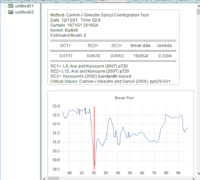
    The addin is straightforward to use. The figure below shows the spool object saving the graph and the table for the results.

    Figure 1
    In Figure 2, similar results have been presented. The difference is that Model E has been used and the pre-whitened results have also been included.  


    Figure 3
    Figure 3 shows the dialog box. You can make your options as you deem appropriate. For example, you can choose any of the methods as shown in Figure 4. Also note that the critical values are not reported. Interested person can see the paper by the authors of the method. Meanwhile, for this method, Carrion-i-Silvestre and Sanso only report the critical values for up to 4 exogeneous variables. Nevertheless, the addin allows you to carry out text for model having more than four exogeneous variables.

    Figure 4

    The criterion in the dialog box is used to select the optimal numbers for leads/lags.

    In the next posts, on cointegration with structural breaks, we shall be looking at all the remaining 3 methods.

    If you find this addin helpful, drop a message or better still follow!!!

    From here, a big thank-you to you.


    Friday, December 10, 2021

    Bootstrap rolling window causality

    Introduction

    A point estimate of causality statistic masks the important question of how the predictive information flows alter as the system undergoes seismic changes. Causal links are, thus, impaired to the extent that they do not account for the inalienable fluctuations or structural breaks in other words. We therefore must accommodate this tendency for the causal relationship to break as the system changes. A simple approach to dealing with this problem of possible changes in the economic structure is to employ time-varying technique, moving window strategy being an attractive method for that purpose. Each time the window is slid across the observations the observations falling within its span are then used to compute causality statistics such as Wald statistic. Balcilar, Ozdemir and Arslanturk (2010) and Nyakabawo, Miller, Balcilar, Das and Gupta (2015), Aye, Balcilar, Bosch and Gupta (2014) have all used this approach, which in a sense can be seen as a time-varying approach.
    As usual, I will simply refer you to those great papers cited in the preceding. Our goal here is to demonstrate how this kind of model can be estimated using Eviews. Suppose we have a bivariate VAR(p), where \(p\) is the optimal lag length selected using the usual criteria. This model is then given by\[\begin{align*}y_{t}=\alpha +\sum_{j=1}^p\theta_{j} y_{t-j}+\sum_{j=1}^p\varphi_{j} x_{t-j}+\epsilon_{t}\\x_{t}=\beta +\sum_{j=1}^p\phi_{j} y_{t-j}+\sum_{j=1}^p\psi_{j} x_{t-j}+\zeta_{t}\end{align*}\]where \(t=1,\dots,T \). But if the evidence of integratedness is found such that \(\kappa=\max(o_x,o_y)\) where \(o_z\) indicates the respective order of integration for variable \(z_t\), then, following Toda and Yamamoto, we can state the model as lag-augmented VAR:
    \[\begin{align*}y_{t}=\alpha +\sum_{j=1}^{p+\kappa}\theta_{j} y_{t-j}+\sum_{j=1}^{p+\kappa}\varphi_{j} x_{t-j}+\epsilon_{t}\\x_{t}=\beta +\sum_{j=1}^{p+\kappa}\phi_{j} y_{t-j}+\sum_{j=1}^{p+\kappa}\psi_{j} x_{t-j}+\zeta_{t}\end{align*}\]The rolling-window sub-samples are defined as \(t=\tau-\ell+1,\tau-\ell,\dots,\tau\), with \(\tau=\ell,\ell+1,\dots,T-\ell,T\) and \(\ell\) is the window size. For each of these sub-samples, causal relationship is tested. 


    Balcilar et al (2010) and Nyakabawo et al (2015) also consider bootstrapping the confidence interval for each sub-sample. While these authors consider the LR statistic to test the hypotheses of causal relationships, the Wald statistic can also be applied. Eviews offers a flexible way to model this relationship and conduct relevant tests. Within the Toda-Yamamoto (T-Y) framework as stated in the second system of equations above, the relevant hypotheses can be conducted. The hypothesis that \(x_t\) does not cause \(y_t\) is given by \(H_0:\varphi_1=\cdots=\varphi_p=0\), while the hypothesis that \(y_t\) does not cause \(x_t\) is given by \(H_0:\phi_1=\cdots=\phi_p=0\). Note that the augmented part of the model specification is not included in the hypothesis as required by the T-Y framework. This implies that the var object in Eviews cannot be applied directly to conduct the T-Y approach to testing causality. At least two efficient ways are available to conduct the T-Y approach to the Granger non-causality testing. I will explain one of them.

    Using the Addin

    Steps using Rolling Causality Addin

    There are few steps to follow in order to carry out rolling causality test using this addin:
    • Estimate a VAR model 
    • Restrict the Model
    • Estimate the Restricted Model
    • Open the Addin and Select the Options as Desired
     After you've done these, the only thing to do again is wait. Yes, depending on the length of the observations, you may have to wait for the addin to do the job. After all, what is tastier than sipping your tea while you wait for the addin to do a great job?


    Estimate a VAR model

    Of course, if you're already familiar with Eviews, you'll agree this is the easiest thing to do on planet earth. There are a couple of ways to do this. But whichever way you choose, just estimate your model. I'm assuming you're using Eviews 10 or latest versions in this post

                                
                                                                        Figure 1

    Restrict and Estimate the Model

    Restring a VAR model in Eviews has been a lot easier since Eviews 10. So, now that the VAR environment is prepared, you can restrict your model seamlessly. In this specification, the optimal lag length is selected to be 7. I do not bother to test for the order of integration, though. I'll say more on this in another post when I discuss the implementation in the Toda-Yamamoto causality. To impose the restrictions, click on the VAR Restrictions tab. In the Restrictions group, the virtual representation of the lags selected will be listed. They are represented as L's. When restricted they have * appended to them as shown in the figure. In this example, I restrict the lags of \(le\) on \(ld\), setting them to zero. In other words, I'm imposing the null hypothesis of no causal effect. This is achieved by inserting 0 in the entry shown. To be sure you're restricting the right parameters, hover the cursor on the entry and the flyover will show that can guide you appropriately. All the lag matrices are correspondingly aligned. Therefore, the same entries in other matrices should be restricted. In Figure 2, the estimated restricted VAR model is shown, with information on the restrictions imposed.

    Figure 2

    To see the effect of these restrictions on the estimated model, you can scroll down. You'll observe that 0's have been imposed on the appropriate entries. If the restrictions are not properly imposed, you can clear the restrictions, using the Clear All button, and then review the restrictions. For this example, Figure 3 shows we're on the right path, with the causal effect of \(le\) sets to nil.

    Figure 3


    Open and Estimate Bootstrap Causality

    Having estimated the restricted model, now is the time to ask the addin to carry out the bootstrap causality. Rolling Bootstrap Causality Test has been integrated to the VAR object. As such, it's listed in the Add-ins for VAR object. To access it, simply click on the Proc tab of the estimated restricted model. Locate the Add-ins on the list that pops up. Follow the right arrow of the Add-ins, There you'll see Rolling Bootstrap Causality Test. These steps are shown in Figures 4 and 5.


    Figure 4

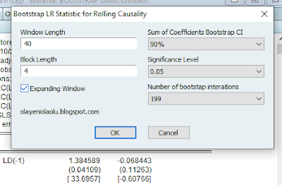
    The addin offers a few options that users can change. Block length can be changed to any desired two-digit number provided that it's less than the number of observations in the sample being used for estimation. Blocking is a way to preserve autocorrelation, that's the sequence of observations that may be particularly of interest in VAR modelling. The window length can be changed too. This is the length of each of the sub-samples used for estimation. But if the Expanding Window checklist is selected, the window length is simply the length of the first sub-sample. Note that expanding window strategy offers a recursive estimation, and the purpose is to review the effect of new information arriving at a later date on causal effects. The confidence interval percentile can be changed too. You can choose any of the four options in the dropdown: 99%, 95%, 90% and 80%. The 90% is the default value. You can also change the level of significance for the p-value plot. 0.05 is the default setting. Lastly, you're offered the opportunity of choosing the desired number of iterations. The default is 199. Other options is there to explore.

    For the example under analysis, the graphs are in Figures 6 and 7 are respectively the LR statistic and its corresponding p-value and the sum of the coefficients for the causal effects. The rolling windows show that the causal effects have change considerably over the years. In some of these years, causal effects are detected where the probability values fall below the critical level of significance (here at 5% level).

                                                                       Figure 6                                     

    Figure 7


    Figure 8

    To implement the bootstrap recursive causality test, I check the option Expanding Window. The following figures report the evolution of causal effects of the arrival of new information. This is found to be significant throughout the estimation period. Figure 9 gives the LR statistic and Figure 10 indicate the behaviour of the sum of the coefficient values on lags of \(le_t\).

    Figure 9

    Figure 10


    Why don't you drop a comment to enhance the capability of this addin? Thanks for your time. 


    Unit root test with partial information on the break date

    Introduction Partial information on the location of break date can help improve the power of the test for unit root under break. It is this ...