Introduction
Nonlinearity is everywhere. To model it, analysts have conjectured in their wildest imagination all manners of techniques. Quantile-on-quantile is one of the latest in the research community. If you haven't seen it applied like most other techniques, it's because it requires a lot of heavy lifting in terms of coding. I have brought you this to ease the burden of using one of the most widely used platforms -- Eviews.Conventionally, quantile regression traces out the effects of the conditional distribution of dependent variable on the dependent variable itself through the impact of the independent variable. It is like asking what the impact of interest rate will be like on inflation if inflation has already reached a particular threshold. Of course, such a question cannot be addressed straightforwardly within the received OLS knowledge. This is where quantile regression stands in to fill the gap.
But then, what about the new estimation strategy quantile-on-quantile regression? Here, both the conditional distributions of the dependent and independent variables modulate the impact of the latter on the former. So, in this case, the question we are interested in is, for example, how extreme inflation (e.g., inflation at say 95 percentile) will respond to extreme interest rate (e.g., at 30-40 percent higher than usual). Put simply, we are interested in how different levels of the independent variable will alter the distribution of the dependent variable. This question cannot be addressed using quantile regression. Because of the existence of two extreme scenarios surfacing within the same policy strategy, the quantile-on-quantile regression comes to the rescue.
QQR is proposed by Sim and Zhou (2015). Yes, it is such a recent method. Again, we are not interested so much in the theory behind this. This can be found in their paper, and I hope the summary here will help you understand that aspect of their paper.
Summary of the method
Let the relationship between \(x_t\) and \(y_t\) be given by\[y_t=\beta^\theta (x_t)+\epsilon_t^\theta\]
Now let \(\tau\)-quantile of \(x_t\) be \(x_t^\tau\). Sim and Zhou suggest the relationship above be approximated by first order Taylor expansion of \(\beta^\theta (x_t)\) around \(x_t^\tau\)
\[\beta^\theta (x_t)\approx \beta_1 (\tau,\theta) + \beta_2 (\tau,\theta)(x_t-x_t^\tau).\]
If follows that
\[y_t= \beta_1 (\tau,\theta) + \beta_2 (\tau,\theta)(x_t-x_t^\tau)+\epsilon_t^\theta\]
At a given value of \(\tau\), the preceding equation can be estimated by quantile regression. Basically, we estimate\[\hat{\beta} (\tau,\theta)=\underset{\beta (\tau,\theta)}{\text{argmin}}\sum_{t=1}^T\rho_\theta \left(y_t - \beta_1 (\tau,\theta)-\beta_2 (\tau,\theta)(x_t-x_t^\tau)\right)\]
where \(\rho_\theta(\cdot)\) is the check function. Rather than estimating this model, the authors realize that there is a need to weight the function appropriately. The reason is that the interest is in the effect exerted locally by the \(\tau\)-quantile of \(x_t\) on \(y_t\). This makes sense in that otherwise the effect will not be contained in the neighbourhood of \(\tau\). They choose the normal kernel function to smooth out unwanted effects that could contaminate the results. The weights so generated are inversely related to the distance between \(x_t\) and \(x_t^\tau\) or, equivalently, between the empirical distribution of \(x_t\), \(F(x_t)\), and \(\tau\). I follow suit in developing the code. Now, the model becomes
\[\hat{\beta} (\tau,\theta)=\underset{\beta (\tau,\theta)}{\text{argmin}}\sum_{t=1}^T\rho_\theta \left(y_t - \beta_1 (\tau,\theta) - \beta_2 (\tau,\theta)(x_t-x_t^\tau)\right)K\left(\frac{(x_t-x_t^\tau)}{h}\right)\]
where \(h\) is the bandwidth. As the choice of bandwidth is critical to getting a good result, in this application, I choose the Silverman optimal bandwidth given by
\[h=\alpha\sigma N^{-1/3}\]
where \(\sigma=\text{min}(IQR/1.34, \text{std}(x))\), \(IQR\) is the inter-quantile range, \(N\) is the sample size and \(\alpha=3.49\).
One snag, however, needs to be pointed out. Eviews does not feature surface plot normally used to present the results in this case. To me, this turns to be an advantage because a more revealing graphical technique has been devised for that purpose. It aligns the boxplots to summarize the results in an equally excellent, if not better, way.
In what follows, I will lead you gently into the world of QQR addin in Eviews
In what follows, I will lead you gently into the world of QQR addin in Eviews
Eviews example
Addin Environment
The QQR addin environment is depicted in Figure 1. If you've already installed the addin, you can click on the Add-ins tab to display the QQR dialogue box as seen below.

Figure 1
The dialogue box is self-explanatory. Three edit boxes are featured. The first one asks you to input the dependent variable followed by a list of exogenous variables. You can include both C and @trend among the exogeneous variables here. However, you should not include the quantile exogeneous variable, which you are required to enter in the second edit box. Note that only one quantile exogeneous variable can be entered here. In the third edit box the period of estimation is indicated.
Example is given in Figure 2. Here, we are estimating the quantile-on-quantile effects of oil price (OILPR) on exchange rate (EXR). We include the third variable, interest rate (INTR). This estimation is carried out over the period of May 2004 and January 2020. Although oil price is an exogenous variable, by entering it in the second variable, we make it the variable whose quantile effect we want to study.

Figure 2
A couple of options are provided. The Coefficient plots category wants you to choose whether to produce the graphs for all the variables in the model or to just produce the graph for the quantile exogenous variable alone. The default is to generate the graphs for all the coefficients in the model. The Graph category wants you to choose to rotate or not the plots. Orientation may count at times. The default is to rotate the plots. Lastly, there is the Plot Label category. How do you want your graphs labelled? On one side or on both sides. It may not matter much. But beauty they say is in the eyes of beholder. I think I love the double-sided label. Hence the default. These categories are boxed with color code in Figure 3.

Figure 3
Graphical Outputs
As noted above, Eviews has yet to develop either the contour or the surface plot usually favored for the quantile-on-quantile result presentations. In the absence of these valuable tools, I opt for boxplot. Boxplot presents the distribution of the data with a couple of details (median, mean, whiskers, outliers and in Eviews confidence interval). But it is a 2-D plot. This means one can only view one side of the object on the x-y plane. To view the other side of the object, one needs to rotate the object. In other words, one needs two 2-D plots to capture some details of the 3-D objects. That is why we have the two plots for one parameter! The graph is named quantileonquantileplot##. The shade indicates 95% confidence interval.
In Figures 4-6, I present the graphs for the three coefficients.

Figure 4

Figure 5

Figure 6
The same results are presented in Figures 7-9 but this time not rotated!
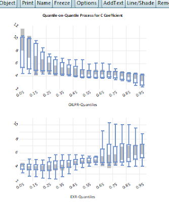
Figure 7

Figure 8

Figure 9
External resources
If one really wants to report the contour or surface plot, there is still hope. Eviews has provided an opportunity to interact with external computational software like MATLAB and R. Since I have MATLAB installed on my system, I simply run the following code in Figure 10. The inputs to the snippet include the matrix and vector objects generated and quietly dumped by the QQR addin in the workfile. They are a19\(\times\)k coefmatrix and a 19-vector taus respectively, where k is the number of parameters estimated.
Figure 10
Figures 11-13 compare the graphs of the estimated coefficients from the QQR addin with those generated using MATLAB. Therefore, you can still estimate your quantile-on-quantile using the Eviews addin as discussed here and have the surface plots for the estimated coefficients done in MATLAB or R. What is more? R is a open source and free.

Figure 11

Figure 12

Figure 13
Requirement
This addin runs fine on Eviews 12. It hasn't been done yet on lower versions.
How to get the addin...
Wondering how to have this addin, are you? Follow this blog!😏 The link is here to download the addin.
Thank you for tagging along.
© 2021 Olayeni Olaolu Richard. Originally published 11/25/2021


