Introduction
A point estimate of causality statistic masks the important question of how the predictive information flows alter as the system undergoes seismic changes. Causal links are, thus, impaired to the extent that they do not account for the inalienable fluctuations or structural breaks in other words. We therefore must accommodate this tendency for the causal relationship to break as the system changes. A simple approach to dealing with this problem of possible changes in the economic structure is to employ time-varying technique, moving window strategy being an attractive method for that purpose. Each time the window is slid across the observations the observations falling within its span are then used to compute causality statistics such as Wald statistic. Balcilar, Ozdemir and Arslanturk (2010) and Nyakabawo, Miller, Balcilar, Das and Gupta (2015), Aye, Balcilar, Bosch and Gupta (2014) have all used this approach, which in a sense can be seen as a time-varying approach.
As usual, I will simply refer you to those great papers cited in the preceding. Our goal here is to demonstrate how this kind of model can be estimated using Eviews. Suppose we have a bivariate VAR(p), where \(p\) is the optimal lag length selected using the usual criteria. This model is then given by\[\begin{align*}y_{t}=\alpha +\sum_{j=1}^p\theta_{j} y_{t-j}+\sum_{j=1}^p\varphi_{j} x_{t-j}+\epsilon_{t}\\x_{t}=\beta +\sum_{j=1}^p\phi_{j} y_{t-j}+\sum_{j=1}^p\psi_{j} x_{t-j}+\zeta_{t}\end{align*}\]where \(t=1,\dots,T \). But if the evidence of integratedness is found such that \(\kappa=\max(o_x,o_y)\) where \(o_z\) indicates the respective order of integration for variable \(z_t\), then, following Toda and Yamamoto, we can state the model as lag-augmented VAR:\[\begin{align*}y_{t}=\alpha +\sum_{j=1}^{p+\kappa}\theta_{j} y_{t-j}+\sum_{j=1}^{p+\kappa}\varphi_{j} x_{t-j}+\epsilon_{t}\\x_{t}=\beta +\sum_{j=1}^{p+\kappa}\phi_{j} y_{t-j}+\sum_{j=1}^{p+\kappa}\psi_{j} x_{t-j}+\zeta_{t}\end{align*}\]The rolling-window sub-samples are defined as \(t=\tau-\ell+1,\tau-\ell,\dots,\tau\), with \(\tau=\ell,\ell+1,\dots,T-\ell,T\) and \(\ell\) is the window size. For each of these sub-samples, causal relationship is tested.
Balcilar et al (2010) and Nyakabawo et al (2015) also consider bootstrapping the confidence interval for each sub-sample. While these authors consider the LR statistic to test the hypotheses of causal relationships, the Wald statistic can also be applied. Eviews offers a flexible way to model this relationship and conduct relevant tests. Within the Toda-Yamamoto (T-Y) framework as stated in the second system of equations above, the relevant hypotheses can be conducted. The hypothesis that \(x_t\) does not cause \(y_t\) is given by \(H_0:\varphi_1=\cdots=\varphi_p=0\), while the hypothesis that \(y_t\) does not cause \(x_t\) is given by \(H_0:\phi_1=\cdots=\phi_p=0\). Note that the augmented part of the model specification is not included in the hypothesis as required by the T-Y framework. This implies that the var object in Eviews cannot be applied directly to conduct the T-Y approach to testing causality. At least two efficient ways are available to conduct the T-Y approach to the Granger non-causality testing. I will explain one of them.
Using the Addin
Steps using Rolling Causality Addin
There are few steps to follow in order to carry out rolling causality test using this addin:- Estimate a VAR model
- Restrict the Model
- Estimate the Restricted Model
- Open the Addin and Select the Options as Desired
After you've done these, the only thing to do again is wait. Yes, depending on the length of the observations, you may have to wait for the addin to do the job. After all, what is tastier than sipping your tea while you wait for the addin to do a great job?
Estimate a VAR model
- Estimate a VAR model
- Restrict the Model
- Estimate the Restricted Model
- Open the Addin and Select the Options as Desired
Of course, if you're already familiar with Eviews, you'll agree this is the easiest thing to do on planet earth. There are a couple of ways to do this. But whichever way you choose, just estimate your model. I'm assuming you're using Eviews 10 or latest versions in this post

Figure 1
Restrict and Estimate the Model
Restring a VAR model in Eviews has been a lot easier since Eviews 10. So, now that the VAR environment is prepared, you can restrict your model seamlessly. In this specification, the optimal lag length is selected to be 7. I do not bother to test for the order of integration, though. I'll say more on this in another post when I discuss the implementation in the Toda-Yamamoto causality. To impose the restrictions, click on the VAR Restrictions tab. In the Restrictions group, the virtual representation of the lags selected will be listed. They are represented as L's. When restricted they have * appended to them as shown in the figure. In this example, I restrict the lags of \(le\) on \(ld\), setting them to zero. In other words, I'm imposing the null hypothesis of no causal effect. This is achieved by inserting 0 in the entry shown. To be sure you're restricting the right parameters, hover the cursor on the entry and the flyover will show that can guide you appropriately. All the lag matrices are correspondingly aligned. Therefore, the same entries in other matrices should be restricted. In Figure 2, the estimated restricted VAR model is shown, with information on the restrictions imposed.

Figure 2

Figure 3
Open and Estimate Bootstrap Causality
Having estimated the restricted model, now is the time to ask the addin to carry out the bootstrap causality. Rolling Bootstrap Causality Test has been integrated to the VAR object. As such, it's listed in the Add-ins for VAR object. To access it, simply click on the Proc tab of the estimated restricted model. Locate the Add-ins on the list that pops up. Follow the right arrow of the Add-ins, There you'll see Rolling Bootstrap Causality Test. These steps are shown in Figures 4 and 5.


Figure 4
The addin offers a few options that users can change. Block length can be changed to any desired two-digit number provided that it's less than the number of observations in the sample being used for estimation. Blocking is a way to preserve autocorrelation, that's the sequence of observations that may be particularly of interest in VAR modelling. The window length can be changed too. This is the length of each of the sub-samples used for estimation. But if the Expanding Window checklist is selected, the window length is simply the length of the first sub-sample. Note that expanding window strategy offers a recursive estimation, and the purpose is to review the effect of new information arriving at a later date on causal effects. The confidence interval percentile can be changed too. You can choose any of the four options in the dropdown: 99%, 95%, 90% and 80%. The 90% is the default value. You can also change the level of significance for the p-value plot. 0.05 is the default setting. Lastly, you're offered the opportunity of choosing the desired number of iterations. The default is 199. Other options is there to explore.
For the example under analysis, the graphs are in Figures 6 and 7 are respectively the LR statistic and its corresponding p-value and the sum of the coefficients for the causal effects. The rolling windows show that the causal effects have change considerably over the years. In some of these years, causal effects are detected where the probability values fall below the critical level of significance (here at 5% level).

Figure 6

Figure 7
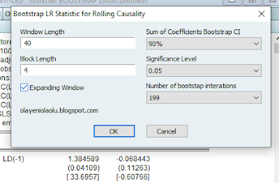
Figure 8
To implement the bootstrap recursive causality test, I check the option Expanding Window. The following figures report the evolution of causal effects of the arrival of new information. This is found to be significant throughout the estimation period. Figure 9 gives the LR statistic and Figure 10 indicate the behaviour of the sum of the coefficient values on lags of \(le_t\).

Figure 9

Figure 10


